Computational Fluid Dynamics (CFD) is about simulating fluids’ behaviour by solving governing equations. Many formulations of such equations are available but they all come from Navier-Stokes equations.
Their derivation from first principle is a long process which is worth studying at least once. I’m going to report here just the final form for finite volumes, precisely the Eulerian integral formulation.
Let’s consider an infinitesimal element with surface \(S\) and volume \(\mathcal{V}\). The equation describing the conservation of mass is
$$
\frac{\textrm{d}}{\textrm{d} t} \iiint_{\mathcal{V}} \rho\;\textrm{d} \mathcal{V} + \iint_{S} \rho (\vec{V} \cdot \vec{n} )\;\textrm{d}S = 0
$$
where \(t\) is the time, \(\rho\) is the fluid density, \(\vec{V}\) is the velocity and \(\vec{n}\) is the surface normal vector. Similar equations can be obtained to balance momentum and energy. In particular, the momentum equation comes from Newton’s second law which states that the rate of change of momentum is equal to the sum of applied forces. The energy equations comes from the principle of energy conservation.
Solving the Navier-Stokes equations for complex geometries is a challenging task and simplified formulations of the equations are solved instead. For example, if viscous effects are modelled with turbulence models, we are solving the Reynolds-averaged Navier-Stokes equations. If viscous effects are neglected completely, we are solving Euler equations.
Too much theory? Well, it’s time to have some fun then! The first step to simulate the flow around an aerofoil is to create the mesh for the CFD solver. For a NACA 0012 aerofoil, we can have an hybrid mesh, produced for example with GMSH for RANS equations.

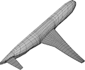
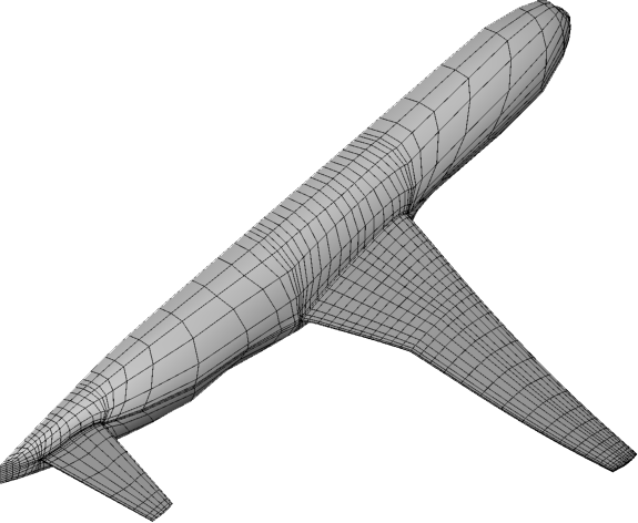
For more complex three-dimensional geometries, it’s wise to rely on CAD software and commercial mesh generator in order to speed up the process. For example, a mesh for the Common Research Model is freely available online for Euler equations and it looks like this:
The next step is to solve the equations using a CFD solver. Commercial programs are widely used but we can use an open-source solver called SU2.
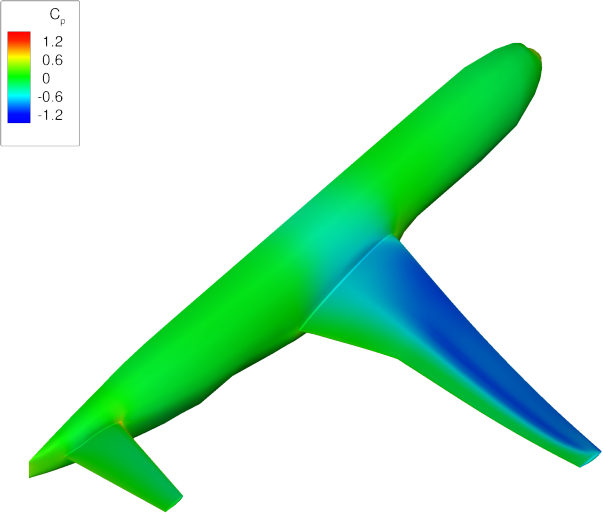
The steady-state solution for the Common Research Model can be depicted with a colourful plot which shows the coefficient of pressure.
This is a very quick tour of CFD. Many interesting things can be achieved by coupling CFD with structural or flight dynamics solvers and usually the CFD mesh must be deformed as well. Good luck with CFD!