It’s possible to match two interesting things: flight dynamics and interactive programming with Python. The magic tool we’re going to use is called Jupyter Notebook. Basically, it’s Python programming done with our favourite web browser.
As we seen in the previous post about flight dynamics, the coupling of rigid body motions and aerodynamics leads to a peculiar aircraft behaviour. Using a Jupyter notebook, we’re going to integrate the equations of motion as function of time. We’ll produce some plots (like the one below!) showing the short and long term response of the airplane.
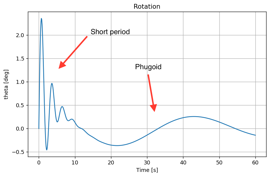
The rigid rotation is shown in this plot. The short term oscillations disappear after few seconds since the short period mode is strongly damped. However, the long term response is dominated by the phugoid mode which has low frequency and little damping.
I’ve included the Jupyter notebook I used to produce this plot here below. The implementation is quite technical but I tried to include some comments to make it easier to read. However, if you are interested, please feel free to contact me!
Fligth dynamics, interactively!
Let’s import some Python modules. We’re going to use some modules from standard library (time, math) but also NumPy and SciPy
import time
import math

# Numpy and Scipy
import scipy as sc
import numpy as np

import scipy.integrate as si

import scipy.linalg as sl
import numpy.linalg as nl

from numpy import pi as pi
from scipy.optimize import fsolve as fsolve

# Matplotlib
%matplotlib inline
import matplotlib.pyplot as plt
import matplotlib.pylab as pylab

pylab.rcParams['figure.figsize'] = (8, 5)
pylab.rcParams['figure.dpi'] = 96
pylab.rcParams['savefig.dpi'] = 96
Parameters
The test case we’re going to implement is taken from literature, specifically from the book “Flight Dynamics Principles” – Cook, M.V., 2nd edition at page 106.
# Units: Imperial

#-------------------------------- General parameters
#- Parameters at sea level: air density and thrust
TSL = 1000
rho0 = 1.10

#- Initial conditions: speed, angle of attack,
#  Euler angle and air density at given altitude
V0 = 305
alpha0 = 0.
theta0 = 0.
zE0  = 0.
rho = 0.00238

#- Mass and inertia properties
mass = 746
Iy = 65000
gravity = 32.2

#-------------------------------- Stability derivatives
# These derivatives represent how the aerodynamic forces
# change due to the flight dynamics unknowns. For example,
# Zw represents the change in the vertical force due to the
# vertical velocity w

#- Derivatives - Z direction
Zu = -159.64
Zu_dot = 0.

Zw = -328.24
Zw_dot = 0

Zq = 0
Zq_dot = 0

Zdelta = -16502.0

#- Derivatives - X direction
Xu = -26.26
Xu_dot = 0.

Xw = 79.82
Xw_dot = 0

Xq = 0
Xq_dot = 0

Xdelta = 0

#- Derivatives - Rotation
Mu = 0
Mu_dot = 0

Mw = -1014.0
Mw_dot = -36.4

Mq = -18135.0
Mq_dot = 0

Mdelta = -303575.0

#-------------------------------- Simulation options
# We are going to simulate the first 60 seconds. The solution to
# the differential equations is calculated each 0.1 seconds

simTime = [0, 60]
simStep = 0.1

# Horizontal and vertical velocity at equilibrium condition
Ue = V0*np.cos(alpha0)
We = V0*np.sin(alpha0)

# Initial conditions. We're going to simulate an initial disturbance
# in the angular velocity q
state_vector0 = [0, 0, 0.1, 0]
elevator0 = 0
throttle0 = 0
Equations of motion
These differential equations express the evolution of the system with respect to time. This is the set of equations that we’ll integrate to get the flight dynamics response of the system.
$$\begin{align}
\left[ \begin{array}{cccc}
m-X_{\dot u} & -X_{\dot w} & -X_{\dot q} & 0\\
-Z_{\dot u} & m-Z_{\dot w} & -Z_{\dot q} & 0 \\
-M_{\dot u} & -M_{\dot w} & I_y-M_{\dot q} & 0\\
0 & 0 & 0 & 1
\end{array} \right]
\left[ \begin{array}{c}
{\dot u} \\
{\dot w} \\
{\dot q} \\
{\dot \theta} \\
\end{array} \right] = &
\left[ \begin{array}{cccc}
X_{u} & X_{w} & X_{q} & 0 \\
Z_{u} & Z_{w} & Z_{q} & 0 \\
M_{u} & M_{w} &M_{q} & 0 \\
0 & 0 & 0 & 0
\end{array} \right]
\left[ \begin{array}{c}
{ u } \\
{ w } \\
{ q } \\
{\theta} \\
\end{array} \right] + \\ &
\left[ \begin{array}{cccc}
0 & 0 & – m W_e & – m g \cos \theta_0 \\
0 & 0 & m U_e & – m g \sin \theta_0 \\
0 & 0 & 0 & 0 \\
0 & 0 & 1 & 0
\end{array} \right]
\left[ \begin{array}{c}
{ u} \\
{ w} \\
{ q} \\
{\theta} \\
\end{array} \right] + \\ &
\left[ \begin{array}{c}
X_\delta \\
Z_\delta \\
M_\delta \\
0
\end{array} \right]
\delta +
\left[ \begin{array}{c}
T_{SL} \frac{\rho}{\rho_0} \\
0 \\
0 \\
0
\end{array} \right] \eta
\end{align}
$$
Matrices and eigenvalues
def getMatrices(Ue, We):
    # This function return the Jacobian matrix of the system
    # and the other vectors related to control surfaces and thrust
    # that we need for the integration

    # ---------
    I1 = np.array([[mass-Xu_dot, -Xw_dot, -Xq_dot, 0.],
                   [-Zu_dot, mass-Zw_dot, -Zq_dot, 0.],
                   [-Mu_dot, -Mw_dot, Iy-Mq_dot, 0.],
                   [      0,       0,        0, 1]])

    In = nl.inv(I1)


    # ---------
    An = np.array([[Xu, Xw, Xq, 0],
                   [Zu, Zw, Zq, 0],
                   [Mu, Mw, Mq, 0],
                   [0,0,0,0]])

    Kn = np.array([[0, 0, - mass * We, - mass * gravity * np.cos(theta0)],
                   [0, 0, + mass * Ue, - mass * gravity * np.sin(theta0)],
                   [0, 0, 0, 0],
                   [0, 0, 1, 0]])

    A = An + Kn

    # ---------
    D = np.array([Xdelta, Zdelta, Mdelta, 0])
    T = np.array([TSL * rho / rho0, 0, 0, 0])

    return np.dot(In, A), np.dot(In, D), np.dot(In, T)
Using the function we have written, we can calculate the eigenvalues of the system. We’re expecting two eigenvalues corresponding to short period and phugoid!
Jac, Jac_D, Jac_T = getMatrices(V0, 0.)

print "Jacobian matrix = "
print Jac
print

print "Eigenvalue analysis: "
evals = nl.eig(Jac)[0]
for ev in evals:
    print "\t", ev
print
Jacobian matrix =
[[ -3.52010724e-02   1.06997319e-01   0.00000000e+00  -3.22000000e+01]
 [ -2.13994638e-01  -4.40000000e-01   3.05000000e+02   0.00000000e+00]
 [  1.19836997e-04  -1.53536000e-02  -4.49800000e-01   0.00000000e+00]
 [  0.00000000e+00   0.00000000e+00   1.00000000e+00   0.00000000e+00]]

Eigenvalue analysis:
	(-0.44586984133+2.16437192886j)
	(-0.44586984133-2.16437192886j)
	(-0.0166306948626+0.147431081456j)
	(-0.0166306948626-0.147431081456j)
Eigenvalues are complex conjugate since they represent harmonic motions. The imaginary part of the eigenvalue is related to oscillation frequency. The eigenvalue with higher frequency is the short period whereas the low-frequency mode is the phugoid.
Literature comparison
The solution to the eigenvalue problem can be derived analitically. The final result is copied here from literature as a comparison with the evaluation we made. In oarticular, transfer function is given as
$$
TF(s) = \frac{-4.664 (s+0.135) (s+0.267)}{(s^2+0.033 s + 0.022) (s^2 + 0.893 s + 4.884)}
$$
with stability modes given by the solution of the denominator
$$
s_1 = -0.0165 \pm 0.1474 \mathrm{i}
$$
and
$$
s_2 = -0.4465 \pm 2.164 \mathrm{i}
$$
As you can see, the numeric evaluation gives very similar results.
Integration
At this point, it is time to integrate the equations and have some nice plots of the flight dynamics response.
def integrate(y0, tSpan, dt, update=None, callback=None, maxInnerSteps=10000):
    '''
    Integrate a set of first order differential equation. This function acts
    similarly to MATLAB's ode45 function.

    t, y, timing = integrate(y0, tSpan, dt, update, callback, maxInnerSteps)

    INPUT
      y0 = initial conditions (y at tBeg)
      tSpan = [tBeg, tEnd]
      dt = step size

      update = fn(t, y)
      callback = fn(t, y) called at every succeful integration

      maxInnerSteps = max number of inner iterations (default: 10000)

    OUTPUT
      t = list of timesteps
      y = solutions at timestep (one line per timestep)
      timing = elapsed time for the integration of the timestep
    '''

    tBegin = min(tSpan)
    tEnd = max(tSpan)

    history_t = []
    history_y = []

    integr = sc.integrate.ode(update)
    integr.set_integrator('dopri5', nsteps=maxInnerSteps)
    integr.set_initial_value(y0, tBegin)

    t_elapsed = []
    tic = time.time()

    history_t.append(tBegin)
    history_y.append(np.array(y0))

    while integr.t < tEnd:
        values = integr.integrate(integr.t + dt)

        if not integr.successful():
            raise Exception("Integration not successful")

        history_t.append(integr.t)
        history_y.append(values)

        if callback is not None:
            try:
                callback(integr.t, values)
            except:
                print "Error in the callback function"

        toc = time.time() - tic
        t_elapsed.append(toc)

    return np.array(history_t), np.array(history_y), np.array(t_elapsed)

def eqsOfMotion(time, state_vector, elevator, throttle, Ue, We):
    """
    This function return the first order derivative of the state vector at each timestep.
    The derivative is calculated using the Jacobian matrix evaluated earlier.
    """

    if np.any(np.isnan(state_vector)):
        raise ValueError("NaN!")

    Jac, Jac_D, Jac_T = getMatrices(Ue, We)

    state_vector_dot = np.dot(Jac, state_vector) \
        + Jac_D * elevator \
        + Jac_T * throttle

    return state_vector_dot
It’s good to output the initial conditions and the initial external disturbance
print "Initial state vector:"
print state_vector0
print

print "Elevator = ", elevator0 * (180./np.pi)
print "Throttle = ", throttle0

fn_integrate = lambda t, x: eqsOfMotion(t, x, elevator0, throttle0, Ue, We)
t_time, t_values, t_elapsed = integrate(np.array(state_vector0), simTime, simStep, fn_integrate, None)

print "Integration performed!"
Results
In this section the integration is performed and four plots are produced as result of the integration. Short period and phugoid are clearly visible in the response of the system.
names = ["u", "w", "q", "theta"]
titles = ["Horizontal speed", "Vertical speed", "Angular speed", "Rotation"]
units = ["[ft/s]", "[ft/s]", "[deg/s]", "[deg]"]
convertion = [1, 1, (180./np.pi), (180./np.pi)]

plt.figure()

for index in range(4):

    plt.figure(index +1)
    plt.plot(t_time, t_values[:,index]*convertion[index])
    plt.ylabel("{} {}".format(names[index], units[index]))
    plt.xlabel("Time [s]")
    plt.title(titles[index])
    plt.grid('on')

plt.show()


Calculating flight path
The flight path can be calculated as post-processing step.
# The derivatives of the horizontal and vertical position in the inertial frame are calculated
xE_dot = +(Ue + t_values[:,0]) * np.cos(t_values[:,3]) + (We + t_values[:,1]) * np.sin(t_values[:,3])
zE_dot = +(Ue + t_values[:,0]) * np.sin(t_values[:,3]) - (We + t_values[:,1]) * np.cos(t_values[:,3])

# When these derivatives are needed at time steps not sampled, we have to use interpolation.
# This is needed because the integration routine can choose time steps for which no evaluation of
# xE_dot or zE_dot is available
def int_path(t, x):
    xE_dot_temp = np.interp(t, t_time, xE_dot)
    zE_dot_temp = np.interp(t, t_time, zE_dot)
    return np.array([xE_dot_temp, zE_dot_temp])

path_time, path_values, _ = integrate(np.array([0,0]), simTime, simStep, int_path, None)

plt.figure()
plt.plot(path_values[:,0], path_values[:,1])
plt.xlabel('Horizontal translation [ft]')
plt.ylabel('Vertical translation [ft]')
plt.title('Flight path')
plt.grid()
plt.show()

Leave a Reply